Case study: visual interface tutorial

Nuno Saraiva-Agostinho

2024-11-18

psichomics is an interactive R package for integrative analyses of alternative splicing and gene expression based on The Cancer Genome Atlas (TCGA) (containing molecular data associated with 34 tumour types), the Genotype-Tissue Expression (GTEx) project (containing data for multiple normal human tissues), Sequence Read Archive and user-provided data. The data from GTEx, TCGA and select SRA projects include subject/sample-associated information and transcriptomic data, such as the quantification of RNA-Seq reads aligning to splice junctions (henceforth called junction quantification) and exons.

Installing and starting the program

Install psichomics by typing the following in an R console (the R environment is required):

install.packages("BiocManager")
BiocManager::install("psichomics")

After the installation, start the visual interface of the program in your default web browser by typing:

library(psichomics)
psichomics()

Exploration of clinically-relevant, differentially spliced events in breast cancer

The following case study was adapted from psichomics’ original article:

Nuno Saraiva-Agostinho and Nuno L. Barbosa-Morais (2019). psichomics: graphical application for alternative splicing quantification and analysis. Nucleic Acids Research.

Breast cancer is the cancer type with the highest incidence and mortality in women (Torre et al., 2015) and multiple studies have suggested that transcriptome-wide analyses of alternative splicing changes in breast tumours are able to uncover tumour-specific biomarkers (Tsai et al., 2015; Danan-Gotthold et al., 2015; Anczuków et al., 2015). Given the relevance of early detection of breast cancer to patient survival, we can use psichomics to identify novel tumour stage-I-specific molecular signatures based on differentially spliced events.

Downloading and loading TCGA data

The quantification of each alternative splicing event is based on the proportion of junction reads that support the inclusion isoform, known as percent spliced-in or PSI (Wang et al., 2008).

To estimate this value for each splicing event, both alternative splicing annotation and junction quantification are required. While alternative splicing annotation is provided by the package, junction quantification may be retrieved from multiple sources.

Start by loading breast cancer data by following these instructions:

1. To load TCGA data, click on the blue panel Download/load TCGA data.
2. Fill in the Tumour type field with Breast invasive carcinoma (BRCA).
3. Set the most recent date available in the Date field.
4. In the Data type field, select Clinical data, Junction quantification and Gene expression (RSEM).

Note there is also the option for Gene expression (normalised by RSEM). However, we recommend to load the raw gene expression data instead, followed by filtering and normalisation as demonstrated afterwards.

5. Confirm if the Folder where data is stored field indicates the appropriate folder to where your browser downloads files.
6. Click Load data. If the required files are not available in the given folder, an information message will appear asking if you want to download the requested data. Click Download data and, when all downloads are finished, load data by clicking on Load data again (do not change any parameters).

Downloading multiple files: Note that multiple files will be requested for download at once. Some web browsers (such as Google Chrome) will ask for your confirmation before allowing such behaviour. In order to proceed, please allow multiple downloads.

Windows limitations: If you are using Windows, note that the downloaded files have huge names that may be over Windows Maximum Path Length. A workaround would be to manually rename the downloaded files to have shorter names, move all downloaded files to a single folder and load such folder by going to Load user files > Folder input and selecting the newly-created folder in Folder where data is stored.

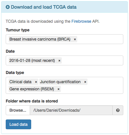
Options to load TCGA data.

After the data finish loading (keep an eye on the progress bar at the top-right corner), the on-screen instructions at the right will be replaced by the loaded data, including options to view and save such data.

Filtering and normalising gene expression

To filter and normalise gene expression, click the green panel Gene expression filtering and normalisation. Within this panel, click the different grey sections (Gene filtering, Normalisation and Compute CPM and log-transform) to check the settings available for processing gene expression. When you are ready to proceed, click Filter and normalise gene expression.

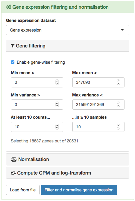
Options to filter and normalise gene expression.

Quantifying alternative splicing

After loading the clinical and alternative splicing junction quantification data from TCGA, quantify alternative splicing by clicking the green panel Alternative splicing quantification.

1. From the loaded data, select the junction quantification dataset to use in Alternative splicing junction quantification. For many tumour types, only one dataset is provided.
2. Select the alternative splicing event annotation Human hg19/GRCh37 (2017-10-20). Note that there are other annotation files available and you can also load custom annotation files.

Custom splicing annotation: Additional alternative splicing annotations can be prepared for psichomics by parsing the annotation from programs like VAST-TOOLS, MISO, SUPPA and rMATS. Note that SUPPA and rMATS are able to create their splicing annotation based on transcript annotation. For more information, read this tutorial.

3. Choose the event type(s) of interest. For the purposes of following the case study, select Skipped exon (SE), Mutually exclusive exon (MXE), Alternative 5’ splice site (A5SS), Alternative 3’ splice site (A3SS), Alternative first exon (AFE) and Alternative last exon (ALE).
4. Set the minimum read counts’ threshold to 10. Inclusion levels calculated with total read counts below this threshold are discarded from further analyses.
5. Click Quantify alternative splicing.

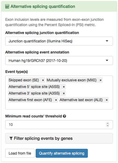
Options to quantify alternative splicing.

Data grouping

In order to group data for downstream analyses, look for the navigation bar on the top and click Groups. In the displayed table, confirm that three groups are automatically present based on the available sample types: Metastatic, Primary solid Tumor and Solid Tissue Normal.

Next, to create groups by tumour stage, click in the field Select attribute and type tumor stage. Select the first hit (it should be patient.stage_event.pathologic_stage_tumor_stage) and click Create group.

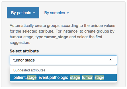
Creating groups by tumour stage.

The table on the right will be updated with the created groups per tumour stage. Next, we will merge tumour stages so as to have only Stage I, II, III and IV. To do so:

1. Select stage i, stage ia and stage ib in the table.

Hint: You can shift-click to select multiple groups at once.

2. Click Merge in the toolbar below the table. A new group named (stage i ∪ stage ia ∪ stage ib) will appear.
3. Select the newly created and the Primary solid Tumor groups and click Intersect to retrieve Tumour Stage I samples.
4. Optionally, rename the newly created group ((stage i ∪ stage ia ∪ stage ib) ∩ Primary solid Tumor) by selecting it and clicking in Rename selected group on the bottom. Type Tumour Stage I and click Rename.

Do the same for tumour stages II, III and IV with their respective subgroups (ignore stage X samples as they are uncharacterised tumour samples). We also recommend to remove groups that are of no interest by selecting them and clicking Remove. In the end, you should end up with a table similar to the one below.

Changing group colours: The colours defined for each group will be used to represent those same groups in the plots throughout psichomics. To change the colour of a given group, select that group and, next to the rename field, change its associated colour (by clicking on the colour field and picking a new colour or by inputting a HEX code) and click Set colour.

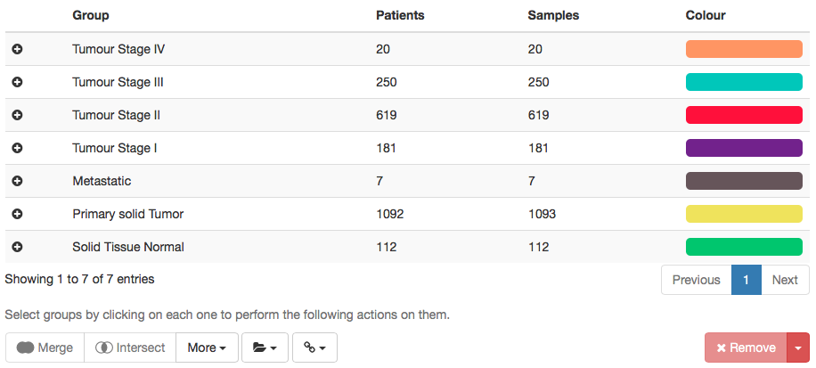
Table showing data groups as created for downstream analyses.

The created groups can then be saved in a text file and loaded in a future session. To do so, in the toolbar below the table click the folder icon (right next to More) and select Save elements from all groups.

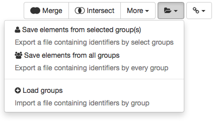
Options to save and load groups.

Principal component analysis (PCA)

PCA is a technique to reduce data dimensionality by identifying variable combinations (called principal components) that explain the variance in the data (Ringnér, 2008). To analyse principal components, click on the Analyses tab located in the navigation menu at the top and select Principal component analysis (PCA).

PCA performance

To perform PCA on alternative splicing data using all samples:

1. In Data to perform PCA on, select Inclusion levels.
2. Select Center values and de-select Scale values.
3. Perform PCA on All samples.
4. Number of missing values to tolerate per event: select 5% of the samples (i.e. 61 samples).

As PCA cannot be performed on data with missing values, missing values need to be either removed (thus discarding data from whole splicing events or genes) or imputed (i.e. attributing to missing values the median of the non-missing ones). This input allows to select the number of missing values that are tolerable per event (i.e. if a splicing event or gene has less than N missing values, those missing values will be imputed; otherwise, the event is discarded from PCA).

5. Perform PCA on All genes and splicing events.
6. Click Calculate PCA.

PCA plotting

After PCA is performed, the Plot PCA panel will automatically open. Note that the explained variance of each principal component (PC) is shown next to the respective component and that PC1 explains most of the data variance, followed by PC2, then PC3, then PC4, etc. The variance plot is also available to compare the explained variance across principal components (by clicking Show variance plot). Now:

1. Select PC1 as the X axis.
2. Select PC2 as the Y axis.
3. In Sample colouring, select Colour using selected groups and in the group selection input insert Tumour Stage I, Tumour Stage II, Tumour Stage III, Tumour Stage IV and Solid Tissue Normal.
4. In Variables to plot in loadings plot, select All variables.

For performance reasons, only the Top 100 variables that most contribute to the select principal components are plotted by default.

5. Click Plot PCA.

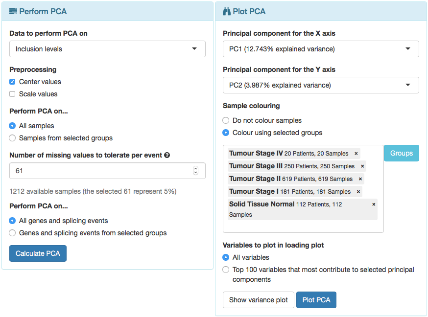
Options to perform and visualise PCA.

Two PCA plots are then rendered. The plot above is a score plot that shows the samples, while the loadings plot below displays the variables (in this case, alternative splicing events). The table below the loadings plot depicts the contribution of each variable to each PC.

Hint: As most plots in psichomics, PCA plots can be zoomed-in by clicking-and-dragging within the plot (click Reset zoom to zoom-out). To toggle the visibility of the data series represented in the plot, click its respective name in the plot legend.

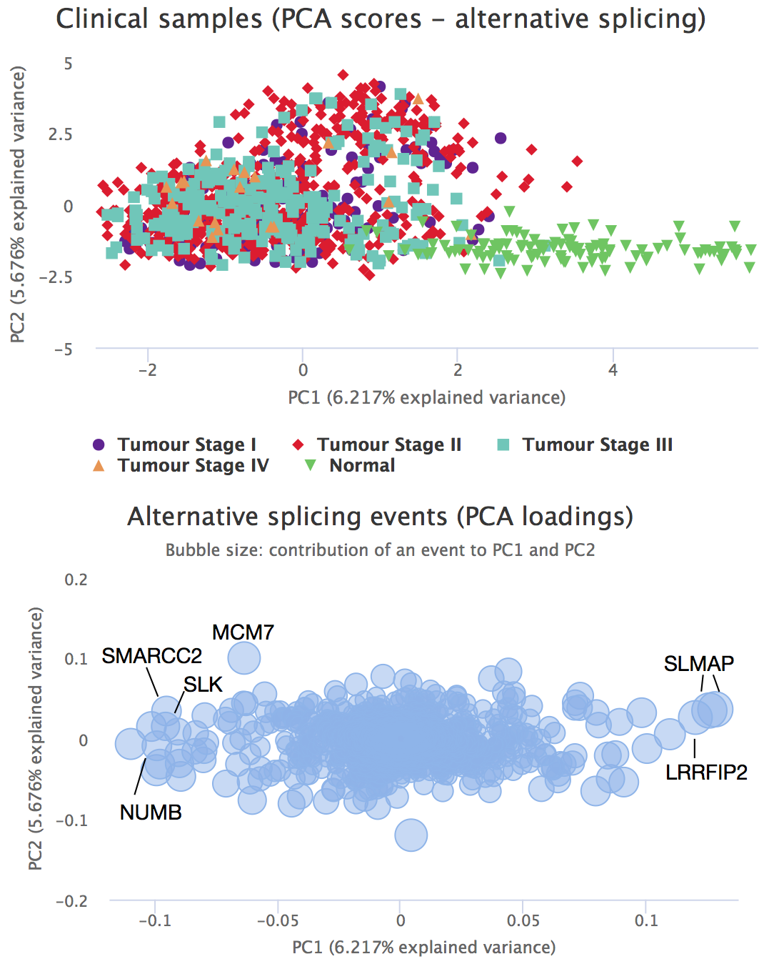
PCA score and loading plots

To perform PCA on alternative splicing data using only Tumour Stage I and Normal samples, click on the blue Perform PCA panel and select to Perform PCA on… Samples from selected groups. In the field that appears, select Tumour Stage 1 and Solid Tissue Normal. Afterwards, click Perform PCA and follow the same steps as before to plot it.

Now, click on one of the events that most contribute to the separation between tumour stage I and normal samples (one of the events with extreme values for the PC1; i.e. the X axis). Differential splicing analysis for that splicing event across selected groups are shown.

To perform PCA using gene expression (both using all samples and only Tumour Stage I and Normal samples), go back to principal component analysis, click in the Perform PCA panel, change Data to perform PCA on to Gene expression (normalised) and follow previous instructions.

NUMB exon 12 inclusion and correlation with QKI gene expression

One of the splicing events that most contribute the separation between tumour stage I and normal samples is NUMB exon 12 inclusion, whose protein is crucial for cell differentiation as a key regulator of the Notch pathway. The RNA-binding protein QKI has been shown to repress NUMB exon 12 inclusion in lung cancer cells by competing with core splicing factor SF1 for binding to the branch-point sequence, thereby repressing the Notch signalling pathway, which results in decreased cancer cell proliferation (Zong et al., 2014).

The identifier for NUMB exon 12 inclusion in psichomics is SE 14 - 73749067 73746132 73745989 73744001 NUMB. On the top right corner, the selected alternative splicing event can be altered by clicking Change…. Click Change… and input the given identifier.

Differential inclusion of NUMB exon 12

In order to check whether a significant difference in NUMB exon 12 inclusion between tumour and normal TCGA breast samples. To do so, go to Analyses > Individual alternative splicing event and click Samples by selected groups. In the group input element, insert the groups Solid Tissue Normal and Primary solid Tumor. Finally, click Perform analyses.

Consistent with the cited article, NUMB exon 12 inclusion is significantly increased in cancer.

Also of interest:

• Hover each group in the plot to compare the respective number of samples, median and variance.
• To zoom in a specific region, click-and-drag in the region of interest.
• To hide or show groups, click on their name in the legend.

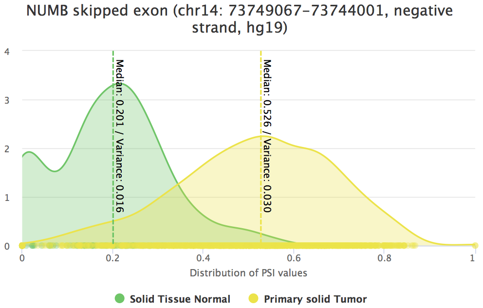
Differential splicing of NUMB exon 12 between tumour and normal samples.

Correlation between NUMB exon 12 inclusion and QKI expression

To check if NUMB exon 12 inclusion is correlated with QKI expression, go to Analyses > Correlation of gene expression and alternative splicing and perform the following:

1. In Gene expression, select Gene expression (normalised).
2. In Gene, type QKI and select the first hit (it may take two seconds for a hit to appear).
3. In Alternative splicing events, remove any alternative splicing events in there, input SE 14 - 73749067 73746132 73745989 73744001 NUMB and select the first hit.
4. Perform correlation analysis on All samples.
5. Correlation method should be set to Spearman’s rank correlation rho.
6. Set the alternative hypothesis to Two-sided.
7. Finally, leave remaining options as default and click Correlate.

According to the obtained results and also consistent with the previous article, the inclusion of the exon is negatively correlated with QKI expression.

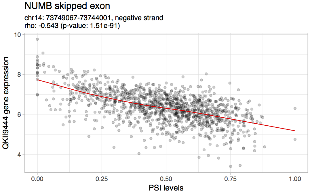
Correlation between NUMB exon 12 inclusion and QKI expression in all TCGA breast samples.

Differential splicing analysis

To analyse differential splicing, click on the Analyses tab located in the navigation menu at the top and select Exploratory (multiple splicing events). Next:

1. Click on the blue panel Perform statistical analyses to open it.
2. In Groups of samples to analyse, click on Samples by selected groups.
3. Select the Tumour Stage I and Solid Tissue Normal groups.
4. In Splicing events to analyse, select All splicing events.
5. Confirm that all statistical analyses are checked.
6. Confirm p-values will be adjusted according to the Benjamini-Hochberg’s method.
7. Click Perform analyses.

When the analyses complete, the results are shown in a plot and in a filterable and sortable table.

Filtering alternative splicing events

Filter events in both the plot and the table by a considerable difference in median between the selected groups (|Δ Median PSI| > 0.1):

1. Click on the blue panel Plot options and table filtering to open it.
2. Click on the X axis tab.
3. Check if Δ Median is selected for the X axis.
4. Click on Highlight points based on Y values and select values lower than -0.1 and higher than 0.1. To do so, input -0.1 in the Lower limit, 0.1 in the Upper limit and check Invert highlighted values.

Next, filter statistically significant splicing events (Wilcoxon q-value ≤ 0.01):

1. Click on the Y axis tab.
2. Select Wilcoxon p-value (BH adjusted) for the Y axis.
3. In Data transformation of Y values, select -log10(|y|).
4. Click on Highlight points based on Y values and change the minimum value to filter significant events. For instance, to consider a p-value of 0.01 or lower, the lower limit should be -log10(0.01), i.e. 2.

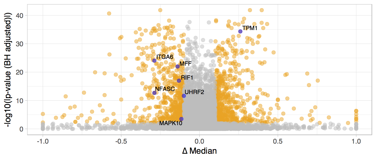
Differentially spliced events (|Δ Median PSI| > 0.1 and Wilcoxon q-value ≤ 0.01). Labelled splicing events have putative prognostic value (more on that in the following section).

The table below is filtered according to highlighted events shown in the plot. If you zoom in the plot (by clicking and dragging), the table will be filtered according to the highlighted events in the zoomed area only (reset zoom to show all highlighted events again). If no events are highlighted, the table presents all events currently shown in the plot.

The table itself is also filterable and sortable. For instance, to sort the table by the difference in variance, click once on Δ Variance. Note that horizontal scrolling is required to visualise all available columns.

The table also provides a column with a density plot of the distribution of the alternative splicing quantification for each event. By clicking on the density plot (or its respective event identifier), a page dedicated to that alternative splicing event’s statistics and exhibiting the density plot in greater detail will show up.

Performing multiple survival analysis

To study the impact of alternative splicing events on prognosis, Kaplan-Meier curves may be plotted for groups of patients separated by the optimal PSI cutoff for a given alternative splicing event that maximises the significance of group differences in survival analysis (i.e. minimises the p-value of the log-rank tests of difference in survival between individuals whose samples have their PSI below and above that threshold).

Given the slow process of calculating the optimal splicing quantification cutoff for multiple events, it is recommended to perform this after filtering the table for differentially spliced events supported by statistical significance.

1. Click on the blue panel Survival analyses by splicing quantification cutoff to open it.
2. Check right data censoring.
3. Use days to death for the follow up time.
4. Use death as the event of interest.
5. In Sample filtering, select Primary solid Tumour (i.e. only use values from tumour samples to perform survival analyses).
6. Select to perform survival analyses based on the Splicing events in current page of the table.
7. Click on Plot survival curves.

Kaplan-Meier plots will appear in the table. Click on the plotted curves to automatically go to the Survival analyses tab, where you can manually adjust the alternative splicing quantification cutoff.

Differential gene expression

Detected alterations in alternative splicing may simply be a reflection of changes in gene expression levels. Therefore, to disentangle these two effects, differential expression analysis between tumour stage I and normal samples should also be performed. To do so, click on the Analyses tab located in the navigation menu at the top and select Exploratory (multiple genes). Next:

1. Click on the blue panel Perform differential expression analyses to open it.
2. In Gene expression dataset, select Gene expression (normalised).
3. Within the Gene-wise linear model fit panel, select the groups Tumour Stage I and Solid Tissue Normal for differential expression.
4. Open the Differential expression statistics panel and check the default settings.
5. Confirm p-values will be adjusted according to the Benjamini-Hochberg’s method.
6. Click Perform analyses.

You can further filter the analyses as previously mentioned for differential splicing analyses.

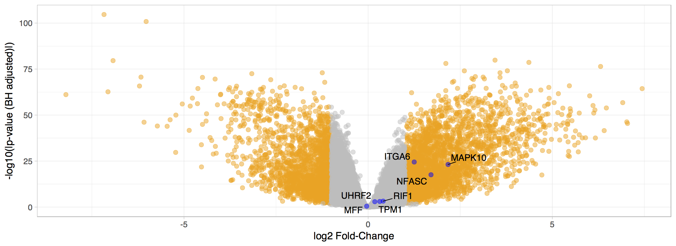
Differentially expressed genes (|log2(Fold-change)| > 1 and FDR ≤ 0.01). Labelled genes are those with alternative splicing events with putative prognostic value.

UHRF2 exon 10 inclusion

One splicing event with prognostic value is the alternative splicing of UHRF2 exon 10. Cell-cycle regulator UHRF2 promotes cell proliferation and inhibits the expression of tumour suppressors in breast cancer (Wu et al., 2012).

The identifier for UHRF2 exon 10 inclusion in psichomics is SE 9 + 6486925 6492303 6492401 6493826 UHRF2. On the top right corner, the selected alternative splicing event can be altered by clicking Change…. Click Change… and input the given identifier.

Differential splicing analysis

In order to test for a significant difference in UHRF2 exon 10 inclusion between tumour stage I and normal samples, go to Analyses > Individual alternative splicing event and click Samples by selected groups. In the group input element, insert the groups Solid Tissue Normal and Primary solid Tumor. Finally, click Perform analyses.

Higher inclusion of UHRF2 exon 10 is associated with normal samples.

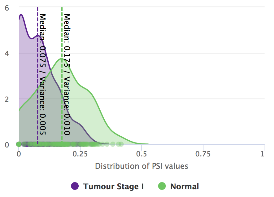
Differential splicing of UHRF2 exon 10 between tumour stage I and normal samples.

Survival analysis

To study the impact of alternative splicing events on prognosis, Kaplan-Meier curves may be plotted for groups of patients separated by a given PSI cutoff for a given alternative splicing event. The optimal PSI cutoff maximises the significance of group differences in survival analysis (i.e.  minimises the p-value of the log-rank tests of difference in survival between individuals whose samples have a PSI below and above that threshold).

To perform survival analysis on a specific event, go to Analyses > Survival analysis.

1. Check right data censoring.
2. Use days to death for the follow up time.
3. Use death as the event of interest.
4. Display time in years.
5. To create groups of patients based on an inclusion levels cutoff, select Inclusion levels cutoff from the selected splicing event.
6. In Sample filtering, select Primary solid Tumor to perform survival analysis using values solely from tumour samples.
7. In the Splicing quantification cutoff, check the value is automatically set to 0.09 (the optimal cutoff).
8. In the Kaplan-Meier plot options, de-select Show censored observations to more clearly display the survival plots.
9. Plot survival curves and fit a Cox proportional hazards (PH) model by clicking on the respective buttons at the bottom.

As per the results, higher inclusion of UHRF2 exon 10 (PSI ≥ 0.09) is associated with better prognosis.

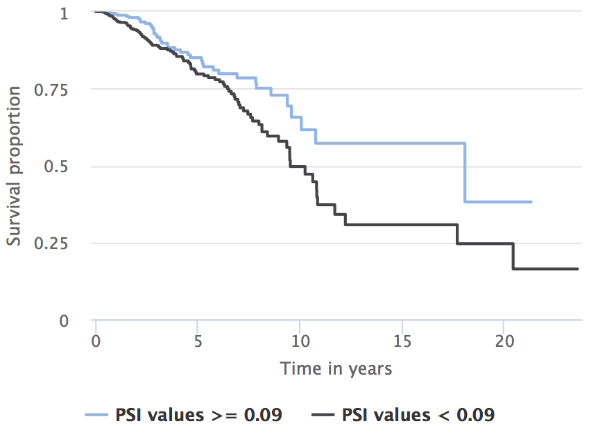
Prognostic value of UHRF2 exon 10 inclusion (patients separated by the optimal PSI cutoff of 0.09).

Differential expression

To check whether alternative splicing changes are related with gene expression alterations, let us perform differential expression analysis on UHRF2. Go to Analyses > Individual gene.

1. Select Gene expression (normalised) for the Gene expression field.
2. In Gene, type UHRF2 and select the first hit.
3. In Groups of samples to compare, select Samples by selected groups.
4. Insert the groups Tumour Stage I and Solid Tissue Normal.
5. Click Perform analyses.

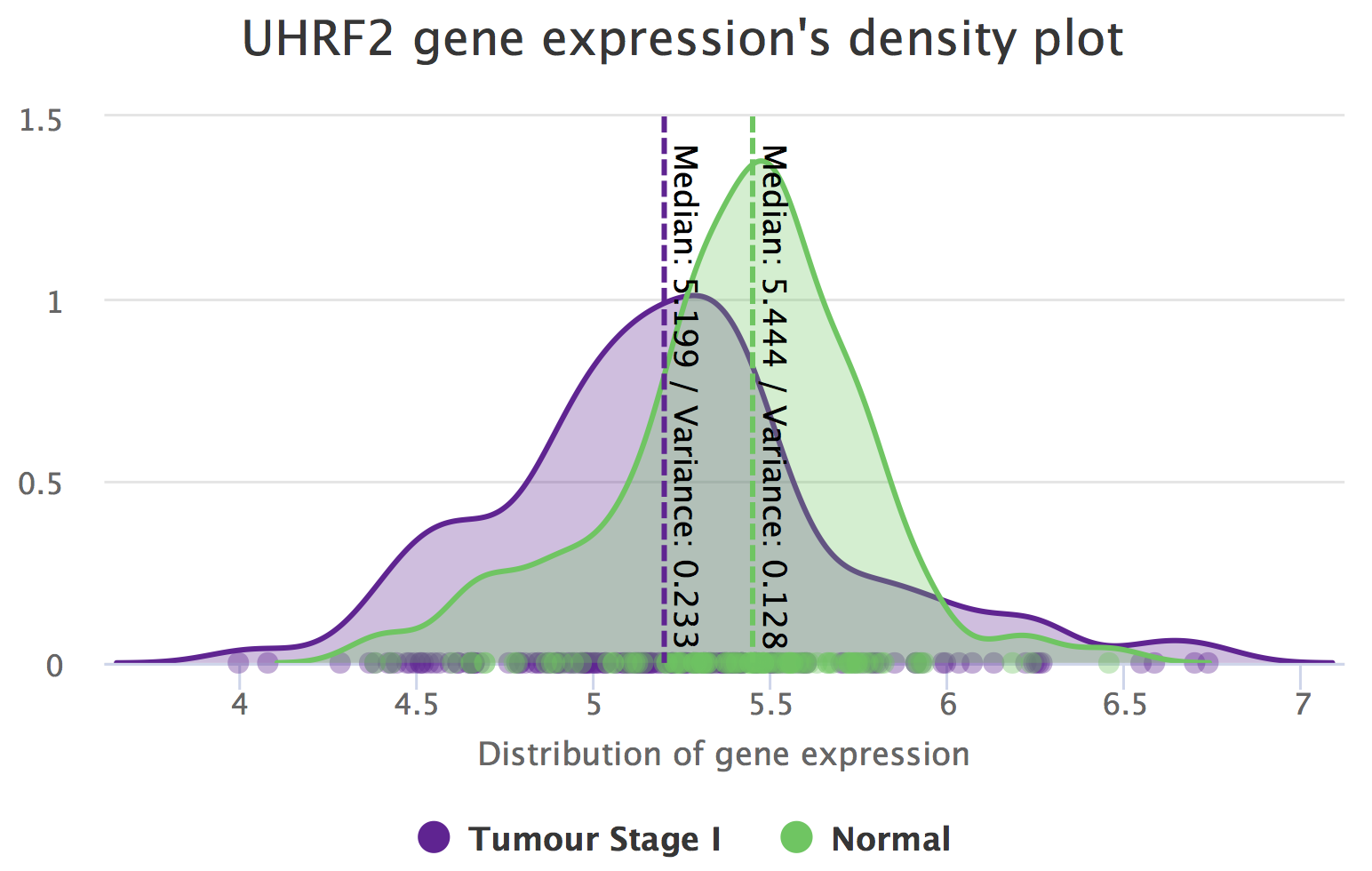
Differential expression of UHRF2 between tumour stage I and normal samples.

It seems UHRF2 is differentially expressed between Tumour Stage I and Solid Tissue Normal. However, going back to exploratory differential gene expression (Analyses > Exploratory (multiple genes)) and looking for UHRF2 (use the Search field above the table), UHRF2 has a log2(|fold-change|) ≤ 1. Following this criterium, the difference in gene expression between these conditions may not be considered biologically relevant.

Survival analysis

To confirm if gene expression has an overall prognostic value, go to Analyses > Survival analysis and perform the following:

1. In the blue Groups for survival analysis panel, select Inclusion levels cutoff from the selected splicing event.
2. Confirm that Sample filtering is only taking into account Primary solid Tumor samples.
3. In Gene expression, select Gene expression (normalised).
4. In Gene, select UHRF2.
5. Wait for the mean and optimal gene expression cutoffs to show up.
6. Click on the optimal cutoff to set it as the cutoff to test.
7. Plot survival curves and fit a Cox proportional hazards (PH) model by clicking on the respective buttons at the bottom.

There seems to be no significant difference in survival between patient groups stratified by UHRF2’s optimal gene expression cutoff in tumour samples (log-rank p-value = 0.279).

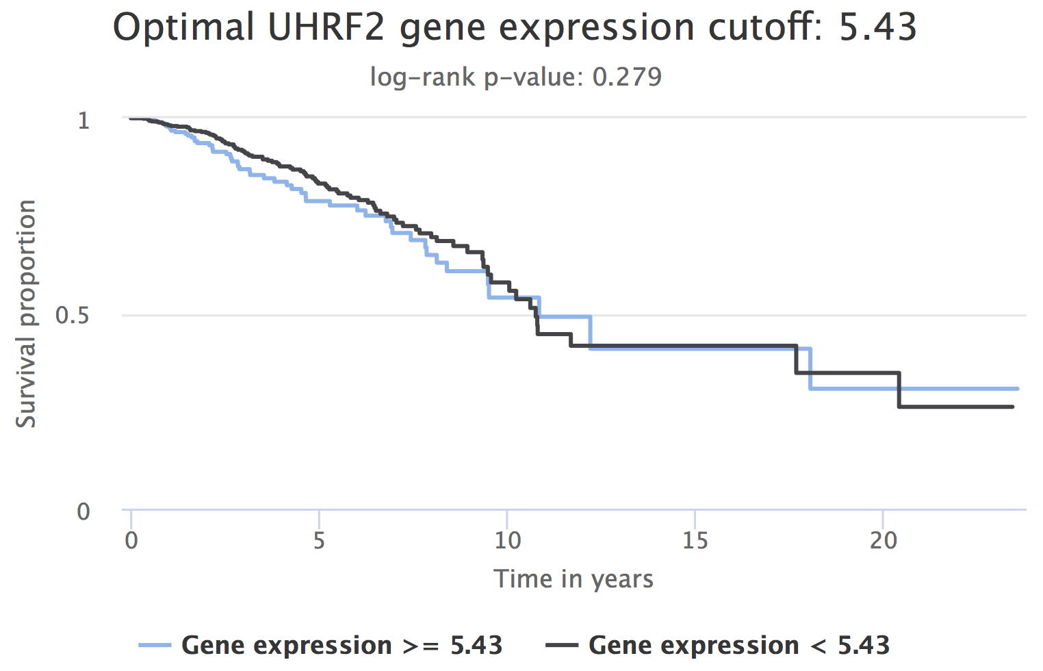
Prognostic value of UHRF2 expression (patients separated by the optimal gene expression cutoff of 5.43).

Literature support and external database information

If an event is differentially spliced and has an impact on patient survival, its association with the studied disease might be already described in the literature. To check so, go to Analyses > Gene, transcript and protein information where information regarding the associated gene (such as description and genomic position), transcripts and protein domain annotation are available.

• The protein plot shows the UniProt matches for the selected transcript. Hover the protein’s rendered domains to obtain more information on them. More information about each protein can be retrieved by clicking the respective UniProt link.
• Links to related research articles are also available. Click Show more articles to be directed to PubMed.
• Multiple links to related external databases are available too:
  • Human Protein Atlas (Cancer Atlas) allows to check the evidence of a gene at protein level for multiple cancer tissues.
  • VastDB shows multi-species alternative splicing profiles for diverse tissues and cell types.
  • UCSC Genome Browser may reveal protein domain disruptions caused by the alternative splicing event. To check so, activate the Pfam in UCSC Gene and UniProt tracks (in Genes and Gene Predictions) and check if any domains are annotated in the alternative and/or constitutive exons of the splicing event.

Interpretation

Higher inclusion of UHRF2 exon 10 is associated with normal samples and better prognosis, and potentially disrupts UHRF2’s SRA-YDG protein domain, related to the binding affinity to epigenetic marks. Hence, exon 10 inclusion may suppress UHRF2’s oncogenic role in breast cancer by impairing its activity through the induction of a truncated protein or a non-coding isoform. Moreover, this hypothesis is independent from gene expression changes, as UHRF2 is not differentially expressed between tumour stage I and normal samples (|log2(fold-change)| < 1) and there is no significant difference in survival between patient groups stratified by its expression in tumour samples (log-rank p-value = 0.279).

Exploring alternative splicing changes between human isogenic stem cells and fibroblasts

Please refer to our methods article:

Nuno Saraiva-Agostinho and Nuno L. Barbosa-Morais (2020). Interactive Alternative Splicing Analysis of Human Stem Cells Using psichomics. In: Kidder B. (eds) Stem Cell Transcriptional Networks. Methods in Molecular Biology, vol 2117. Humana, New York, NY

Load SRA and user-provided local files

Although only select SRA projects are available to be automatically downloaded (based on pre-processed data from the [recount2][recount2] project), other SRA projects can be manually downloaded, aligned using a splice-aware aligner and loaded by the user, as per the instructions in Loading SRA and user-provided RNA-seq data. Sample-associated files from SRA are also supported.

Feedback

All feedback on the program, documentation and associated material (including this tutorial) is welcome. Please send any suggestions and comments to:

Nuno Saraiva-Agostinho (nunoagostinho@medicina.ulisboa.pt)

Disease Transcriptomics Lab, Instituto de Medicina Molecular (Portugal)

References

Anczuków,O. et al. (2015) SRSF1-Regulated Alternative Splicing in Breast Cancer. Molecular Cell, 60, 105–117.

Danan-Gotthold,M. et al. (2015) Identification of recurrent regulated alternative splicing events across human solid tumors. Nucleic Acids Research, 43, 5130–5144.

Ringnér,M. (2008) What is principal component analysis? Nature biotechnology, 26, 303–304.

Torre,L.A. et al. (2015) Global cancer statistics, 2012. CA: a cancer journal for clinicians, 65, 87–108.

Tsai,Y.S. et al. (2015) Transcriptome-wide identification and study of cancer-specific splicing events across multiple tumors. Oncotarget, 6, 6825–6839.

Wang,E.T. et al. (2008) Alternative isoform regulation in human tissue transcriptomes. Nature, 456, 470–476.

Wu,J. et al. (2012) Identification and functional analysis of 9p24 amplified genes in human breast cancer. Oncogene, 31, 333–341.

Zong,F.-Y. et al. (2014) The RNA-binding protein QKI suppresses cancer-associated aberrant splicing. PLoS genetics, 10, e1004289.